

Multi Component Receivers
Technology during the late 1990’s underwent major advancements notably by organisations such as Scripps Institution of Oceanography (Constable et al., 1998). The MCSEM method uses receivers modeled on marine magnetotelluric instrumentation from this period. Receivers have a number of recording devices, including a digital magnetic compass/tilt-meter which records the orientation, a timing system which is synchronised pre and post deployment and magnetic and electric sensors recording multiple axial directions. Receivers record magnetic and electric field time series data. The horizontal electric field receivers are composed of silver-silver chloride electrodes which are between 1 m and 10 m in length (Pethick, 2008). A vertical electric dipole measures the vertical field component and is typically much shorter
and light weight (i.e., the Mk II/III Scripps receiver contains a 1.5m long vertical dipole) (Constable, 2013). The magnetic field is typically recorded by light weight induction coil magnetometers (Key, 2003) (See Figures 1 and 2 The typical components which are detected by commercial designs are x and y magnetic and x, y and vertical electric field directions. The vertical magnetic field is insensitive to thin resistors such as hydrocarbon. The magnetic field sensor is also heavy and its addition to the receiver greatly increases cost. Many commercial operators omit this sensor from their equipment as a consequence of this.
There are numerous receiver parameters to be considered when choosing the most suitable receivers for the survey (as seen in Table 1). Key attributes to consider when planning a CSEM survey include the noise floor of the instrument, timing calibration, timing stability, battery type and energy use, recording capacity, response calibration, navigation and seafloor orientation. Receiver navigation can be poor (e.g., receivers positioned greater than 5 m accuracy) and can introduce measurable variation (i.e., greater than 1%) at short offsets. The electronic dynamic range of instrumentation is important because of large variations in the signal strength. For instance, electric field voltages can range several orders of magnitude (i.e., to
to or lower). 24-bit analogue to digital converters with pre-amplifiers enable high resolution data to be recorded at all source-receiver offsets without signal saturation (Phillips, 2007).
| Receiver Features |
Typical Attributes |
| Magnetic Field Noise Floor |  (at 0.1Hz) (at 0.1Hz) |
| Timing Stability |  in in  intervals result in drift ( intervals result in drift ( /day) /day) |
| Battery Capacity | 6-18 days of continuous logging |
| Storage Capacity |  |
| Receiver Dipole Arm Length |  |
| Electric Field Receivers |  and and  |
| Magnetic Field Receivers |  |
| Sampling Frequency |  |
| Dynamic Range |  |
| Sensitivity |  |
| Depth Rating |  |
| Other Recording Devices | Temperature sensor, magnetic compass, Inclinometer, Horizontal magnetic field channels |
Table 1: Typically encountered receiver features and attributes. These values have been taken from two commercial contractors, OHM’s EFMALS III (OHM, 2008) and WesternGeco (WesternGeco, 2008) receivers.
The main source of electric field receiver noise above 1 Hz is caused by amplifier and electrode induced noise rather than ambient noise (Constable and Weiss, 2006 and Hoversten et al., 2006). There is an inverse relationship between the noise level of electric field receivers and the frequency. For example OHM’s EFMALS III, has a noise floor of  (MacGregor et al., 1998). The receiver can detect and resolve smaller amplitudes for higher frequencies. Most MCSEM receivers have a electric field noise floor around
  and
and  at 1 Hz for magnetic fields assuming a source dipole length of 300 m and a transmission current of 500 A (i.e., 150,000Am2). The total noise is given by equation 2 and the electric field noise floor (3) is the total noise normalized by transmitter moment and receiver electrode dipole arm length:
Equation 2 : 
Equation 3 : 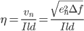
where,
 −Total noise
 −Internal amplifier noise (
 )
)
 − Dipole arm length(
 )
)
 − Electric receiver field noise floor (
 )
)
 − Current(
 )
)
 − Transmitter dipole length()
At 0.1 Hz the average recording period is 10 s and the total noise (vn) is RMS. Commercial EM receivers operate with an electric dipole arm length of 8 to 10 m, however newer lower noise models have been developed to operate with an electrode spacing of 1 m (Quasar, 2012). Their receiver is seen in Figure 3. Commercial operators transmit a high amplitude current in excess of 1000 A at peak output. The higher the transmitter moment, ( , where is a transmitter length and is current) the better the signal to noise. The noise floor for a 100 m long transmitter operating at 1000 A is
  at 0.1 Hz is given by equation (3). This electric field noise floor is close to the values achieved in very deep water marine CSEM surveys. The antenna length can be extended to improve the signal to noise ratio of the receiver. This voltage is proportional to the receiver dipole length (Flosadattir and Constable, 1996). Synchronous stacking can be also used to recover a repetitive signal from the random ambient or instrument noise. The limits and features of electromagnetic systems over next few decades will improve with technological advancements. Hence the features seen in Table 2 should only be taken as a guide. In summary, the main features to consider when planning a survey are the noise threshold of both the E-Field and B-Field sensors and which electric and magnetic axial directions the device will record.
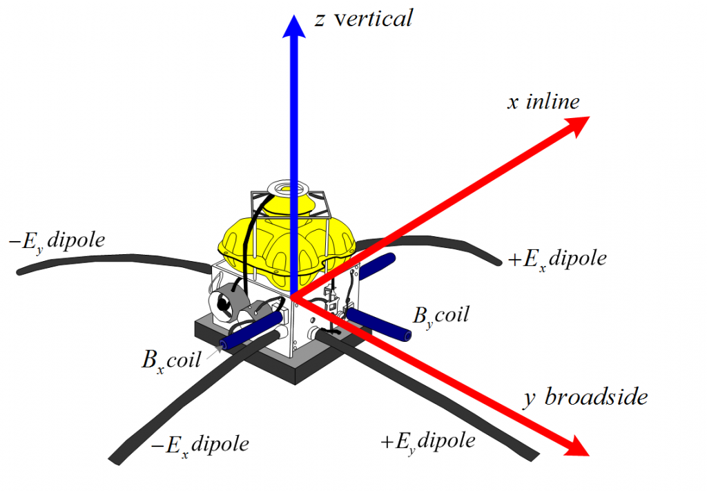
Figure 1: Diagram of a typical marine CSEM multicomponent receiver. The receiver is the Scripps Institution of Oceanography Mark III design, which only records inline magnetic and electric fields and crossline electric field (reproduced from Constable et al., 1998 and Key, 2003)

Figure 2: A receiver from the Scripps Institution of Oceanography. The receiver has all components except the vertical magnetic field. This image was obtained aboard the Scripps Institution of Oceanography’s ship, R.V. Roger Revelle, 2008.

Quasar’s low noise MCSEM receiver. Quasar Geophysical Technologies took an
underwater sensor they developed for the U.S. Navy and redesigned it for ocean bottom surveying with its QMax EM3 underwater electromagnetic receiver (Quasar, 2012). It is the only ocean bottom CSEM receiver to contain all six electric and magnetic components. This image was obtained aboard the Scripps Institution of Oceanography’s ship, R.V. Roger Revelle, 2008.
References
Constable, S. (2013). Review paper: Instrumentation for marine magnetotelluric and controlled source electromagnetic sounding. Geophysical Prospecting 61, 505–532.
Constable, S. and C. J. Weiss (2006). Mapping thin resistors and hydrocarbons with marine em methods: Insights from 1d modeling. Geophysics 71 (2), G43–G51.
Constable, S. C., A. S. Orange, G. M. Hoversten, and H. F. Morrison (1998). Marine magnetotellurics for petroleum exploration; part i, a sea-floor equipment system. Geophysics 63 (3), 816–825.
Flosadattir, A. and S. Constable (1996). Marine controlled-source electromagnetic sounding 1. modeling and experimental design. J. Geophys. Res. 101 (B3), 5507–5517.
Hoversten, G. M., F. Cassassuce, E. Gasperikova, G. A. Newman, J. Chen, Y. Rubin, Z. Hou, and D. Vasco (2006). Direct reservoir parameter estimation using joint inversion of marine seismic ava and csem data. Geophysics 71 (3), C1–C13.
Key, K. (2003). Application of Broadband Marine Magnetotelluric Exploration to a 3D salt Structure and a Fast-Spreading Ridge. Ph. d.
MacGregor, L. M., S. Constable, and M. C. Sinha (1998). The ramesses experiment iii. controlled-source electromagnetic sounding of the reykjanes ridge at 57°45’n. Geophysical Journal International 135 (3), 773–789.
OHM (2008). Ohm surveys. www.ohmsurveys.com.
Pethick, A. (2008). Planning and 4D Visualisation of the Marine Controlled Source Electromagnetic Method. Honours thesis.
Phillips (2007). Feasibility of the Marine Controlled Source Electromagnetic Method for Hydrocarbon Exploration. B.sc.
Quasar (2012). Quasar geo. www.quasargeo.com.
WesternGeco (2008). Westerngeco. http://www.westerngeco.com/content/services/electromagnetic/wgem.asp?