

TBC
CSEM Noise Sources
The success of an MCSEM survey depends on many factors including electromagnetic sources of noise. Amundsen et al. (2006), Maao and Nguyen (2010), Ziolkowski and Wright (2010) cover some aspects of the noise sources found in CSEM. These noise sources include sea water currents, magnetotelluric activity, bipole vibration, internal electrode and amplifier noise and cultural effects, as seen in Table 1 and Figure 1. It should be noted that there is disagreement as to whether the air wave effect is a noise source or a legitimate signal. Amundsen et al. (2006) have suggested it is a noise to remove from data while others have suggested that this effect could be utilised (e.g., Wirianto et al., 2011).
MacGregor (2006) and Constable (2010) have stated that vibrations of the dipole receiver arms can induce an unwanted signal. A vibration of less than 1 mm for a 10 m dipole can produce an induced voltage comparable to the target signal. These movements can be limited by using bottom weights, weighting each electric receiver dipole arm with glass rods and by using farings on dipole arms.
Spheric noise and ocean induced fields can contaminate the received data at lower frequencies ( in transmitter to become oblique or vary in azimuth. This situation should be avoided or the transmitter orientation must be taken into consideration when processing, performing modelling or inversions. Noise sources including “air-wave”, cultural noise, spherics, dipole arm vibrations and water currents must be all considered when dealing with MCSEM data.
| Noise Source | Description |
| Seafloor currents (<1Hz) | The motion of a conductor in an electric field will induce a voltage |
| Spherics (<1Hz) | Lightning and ionic field disturbances resulting in low frequency noise. Spheric noises reduce with water depth. |
| Cultural | Highly conductive or resistive materials close to the receiver will skew the recorded signal |
| Bipole vibration | Vibrations of the electric dipole receiver arms can induce a voltage comparable to the target signal |
| Internal electrode and amplifier noise(>1Hz) | The instrument’s internal noise |
Table 1: A list of MCSEM noise sources to consider
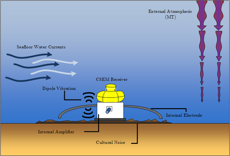
Figure 1 : Overview of standard MCSEM noise sources. Noise sources can be split into two areas, external and internal. Internal sources are within the instruments which are internal amplifier and electrode noise, whilst external noises are caused by seafloor water currents, magnetotelluric (MT) signals, dipole vibration and cultural noises. It is best to conduct a survey in deep water to reduce the effect of seafloor water currents and external atmospheric noise.
Target Style Considerations
The geo-electrical environment effects target detectability and must be considered. Considerations include water depth, target depth, geological type of target, reservoir style, resistivity contrast, resistive non-hydrocarbon geological targets, reservoir complexity and the purpose of the survey (Peace, 2005). Peace (2005), Pethick (2008), Orange et al. (2009), Sasaki and Meju (2009) and Weidelt (2007), have covered the factors influencing the detectability of a target. Water depth and bathymetry is one of the biggest factors influencing detectability. The bathymetry influences the onset of the airwave which may mask a hydrocarbon response. Water bottom channels, canyons and sloping or having the target sit above the water bottom when surveying off a shelf edge will influence the survey Pethick (2008). Water channels and canyons can produce lateral water current flow which can cause transmitter feathering and movement of receiver electrodes. Secondly, the target depth from the water bottom and aerial size of the target compared to the depth affects the detectability of the target. Targets smaller in aerial size in comparison to their depth are harder to detect. Thirdly, the geological type and shape of the target influences the receiver response on the ocean floor. Resistivity contrast also influences a survey plan. If the resistivity contrast between the hydrocarbon and the host is insufficient, it will be unlikely that the survey could detect the hydrocarbon. Resistive structures which are not a result of hydrocarbon, such as salt diapirs, could also lead to false positives. Therefore it is necessary to model a range of geological settings. Salinity and water temperature influences the resistivity of the water column (Orange et al., 2009). Lateral variation caused by salinity cells or temperature variation will greatly influence inversions requiring the water column to be structured as 1D layering. Lastly, the purpose of the survey influences the final survey design. For example, recognisance surveys utilise widely spaced receivers and transmitter lines to target hydrocarbons. 3D surveys use many closely spaced receivers and densely positioned transmitter line locations at multiple azimuths to characterize or appraise a known field Pethick (2008). All geological and survey considerations are encapsulated in Figure 2.
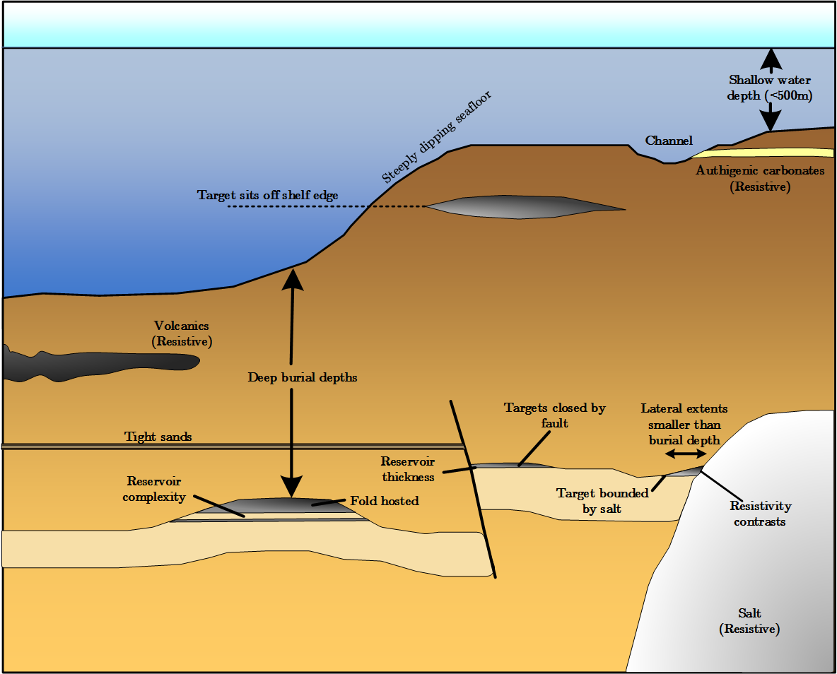
Figure 2 : Geological considerations for MCSEM survey planning.
Seawater Conductivity
Seawater constitutes a large and important element of the geoelectric framework relevant for MCSEM surveying. Determining the correct seawater conductivity is important for both forward modelling and inversion. The conductivity of the sea water varies in the water column and also in the seabed structure itself. Auxiliary instruments record seawater conductivity over the duration of most MCSEM surveys (an example can be seen in 1-5). Sea water varies in resistivity due to temperature, salinity and pressure as described in equation 1.2. The largest variation in sea water conductivity occurs at the near surface (i.e., less than 200 m depth). The sharp gradient in the thermocline is due to temperature variation with depth. Myer et al. (2012) have measured this temperature variation and demonstrates the importance of incorporating this effect in any uncertainty analysis.
Equation 1 : 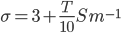
where,
 - Seawater conductivity (
 )
)
 - Seawater temperature (degrees
  )
)
Sea water conductivity is around at  m , typical ocean floor temperatures and reaches a minimum conductivity of
 m at
m at  . This large variation in conductivity has a significant effect on the bulk resistivity of the formation. Archie’s (1942) law can be used to find the saturated formation’s true resistivity in
  · m (see equations 2 and 3).
Equation 2 : 
Equation 3 : 
where,
 - Formation Factor
 - Formation resistivity when 100% saturated with brine
 - Fluid resistivity
 - Formation resistivity when 100% saturated with fluid resistivity
 - Porosity
 - Cementation factor (between 1.3 and 3)
 - Tortuosity factor
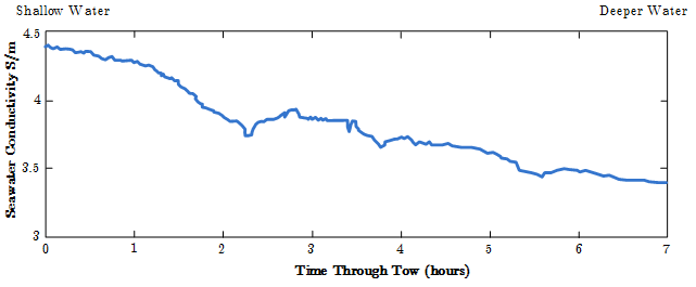
Typical seawater conductivity measurement over the duration of a typical MCSEM survey. The conductivity varies over time and position. The recorded data should be incorporated into the geoelectric model for forward modeling or inversion. Reproduced from MacGregor (2006).)
References
Amundsen, L., L. Laseth, R. Mittet, S. Ellingsrud, and B. Ursin (2006). Decomposition of electromagnetic fields into upgoing and downgoing components. Geophysics 71 (5), G211–G223.
Archie, G. (1942). The electrical resistivity log as an aid in determining some reservoir characteristics. Transactions of the AIME 146 (1), 8.
Constable, S. (2010). Ten years of marine csem for hydrocarbon exploration. Geophysics 75 (5), 75A67–75A81.
Kong, E.N.; Westerdahl, H. E. S. E. T. J. S. (2002). Seabed logging: A possible direct hydrocarbon indicator for deepsea prospects using em energy. Oil and Gas journal 100, 6.
Maao, F. A. and A. K. Nguyen (2010). Enhanced subsurface response for marine csem surveying. Geophysics 75 (3), A7–A10.
MacGregor, L. M. (2006). Ohm short course.
Myer, D., S. Constable, K. Key, M. E. Glinsky, and G. Liu (2012). Marine csem of the scarborough gas field, part 1: Experimental design and data uncertainty. Geophysics 77, 281.
Orange, A., K. Key, and S. Constable (2009). The feasibility of reservoir monitoring using time-lapse marine csem. Geophysics 74 (2), F21–F29.
Peace, D. (2005, 2 May). How to plan for a successful c.s.e.m. survey.
Pethick, A. (2008). Planning and 4D Visualisation of the Marine Controlled Source Electromagnetic Method. Honours thesis.
Sasaki, Y. and M. A. Meju (2009). Useful characteristics of shallow and deep marine csem responses inferred from 3d finite-difference modeling. Geophysics 74 (5), F67–F76.
Weidelt, P. (2007). Guided waves in marine csem. Geophysical Journal International 171 (1), 153–176.
Wirianto, M., W. A. Mulder, and E. C. Slob (2011). Exploiting the airwave for time-lapse reservoir monitoring with csem on land. Geophysics 76 (3), A15–A19.
Ziolkowski, A. and D. Wright (2010). Signal-to-Noise Ratio of CSEM data in Shallow Water, pp. 685–689.