

What is the Airwave
The airwave is a complex interference effect between the air, water and seabed layering. The airwave poses problems for MCSEM surveys because it masks the received the seabed signals at far offsets (Eidesmo et al., 2002). It can be identified by a gradient break in inline electric field profiles and there is also a total phase lag which is dependent on the offset and water depth (Eidesmo and Ellingsrud, 2002). The airwave is affected by the transmitter-receiver offset, transmitter dipole orientation, transmission frequency, resistivity structure and the water depth.
Mitigating the Airwave
Eidesmo and Ellingsrud (2002); (Eidesmo et al., 2002); Wirianto et al. (2011) have offered solutions to the airwave problem but none offer a ’silver bullet’ solution. It is an ongoing problem for industry. The companies EMGS, OHM and Fugro Electro Magnetic are working to resolve it by using various data processing techniques and by limiting its effect by using novel acquisition practices (Ellingsrud et al., 2002). Possible solutions to the airwave problem include selecting acquisition parameters that limit the generation of an airwave, signal processing and even using information in the airwave (Weidelt, 2007). The company, PGS, has claimed to have mitigated the airwave by transmitting and measuring in the time domain. This has reduced the problems associated with the airwave masking deeper responses, but the air wave is still present in the data and can mask subocean responses given the right conditions. Forward modelling should be performed to provide the airwave influence prior to surveying (Mittet, 2004 and Johansen, 2005).
Constable and Weiss (2006) have suggested that the air wave effect can be reduced by utilizing a vertical dipole transmitter. Air-water interface coupling is influenced by transmitter orientation. Horizontal current loops create poloidal magnetic (PM) modes which will enhance the air-water interface coupling (i.e., stronger air wave effect), while vertical current loops create transverse magnetic (TM) modes which reduce the airwave’s influence (MacGregor, 2006) (See Figure 1).
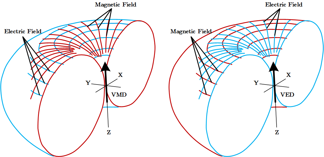
Figure 1: The magnetic and electric field patterns from vertical electric (VED) and magnetic (VMD) dipoles. Horizontal current loops strongly couple with the air-water interface resulting in a large air wave response. The airwave phenomenon can be minimised by using a vertical electric dipole. Reproduced from MacGregor, 2006.
Airwave Onset
Transmission frequency also affects air wave onset and amplitude (Eidesmo et al., 2002). Eidesmo et al. (2002) found that higher transmission frequencies have a larger airwave effect. They also found that the higher frequencies result in shorter onset air-waves (as seen in Table 1). Therefore the benefits of low frequency must be balanced against reduced resolution. The maximum depth of investigation before contamination of the airwave can be calculated by using localization Eidesmo et al. (2002). The depth at which this occurs can be calculated by multiplying the scale factor from Equation 1 ( ) with the water depth (Tompkins et al.,2004). For example, if = 1.76 and the water depth is 1000 m, then the maximum depth of investigation would be 1760 m.
Equation 1 : 


where,
 - Seawater conductivity
 - Sediment conductivity
- Unitless scale factor
| Water Depth(m) | 0.25Hz | 0.5Hz | 1.0Hz | 2.0Hz |
| 500 | 4.8 | 4.0 | 3.4 | 3.0 |
| 600 | 5.2 | 4.3 | 3.9 | 3.5 |
| 700 | 5.7 | 4.7 | 4.3 | 3.8 |
| 800 | 6.1 | 5.0 | 4.6 | 4.1 |
| 900 | 6.5 | 5.4 | 4.9 | 4.5 |
| 1000 | 6.9 | 5.8 | 5.4 | 4.9 |
| 1200 | 7.6 | 6.7 | 6.1 | 5.6 |
| 1400 | 8.5 | 7.5 | 6.8 | 6.2 |
| 1600 | 9.3 | 8.3 | 7.5 | 7.1 |
| 1800 | 10.1 | 9.0 | 8.3 | 7.8 |
| 2000 | 11.0 | 9.8 | 8.9 | 8.4 |
Table 1 : The distance from the source (in km) at which the airwave starts to dominate the overall response. The point at which the response is dominated by the airwave is represented as function of water depth and the signal frequency. Reproduced from Eidesmo et al. (2002).
Understanding the Airwave using Streamlines
In reality, electromagnetic field propagation is extremely complex. Everything in the earth influences the recorded electromagnetic response, from the highly resistive air to the most seemingly insignificant conductive brine filled sandstone unit. Everybody has a preferred method to understanding electromagnetic field behaviour. It could be mathematically, rules of thumb or with static field lines. I like the idea of streamlines as they are able to visualise simulated electric, magnetic and Poynting vector field lines in time. Each to their own.
Streamlines represents flow and flow paths, so for ease of interpretation
- the electric field can be considered to visualize the direction of the flow of charged particles
- the magnetic field the direction of the force on moving charged particles
- the Poynting vector the flow of energy flux.
A static interpretation guide is shown below. The electric field streamlines show the airwave as an interaction between two vortices; the earth vortex and air vortex. The centre of the earth vortex corresponds with the electric x phase inflection point a significantly small amplitude. The air wave front (per indicated by the dashed red line) represents the point where the contribution of “earth” and “air” energy flow is equal. That is above the line is predominantly air wave energy and below the line predominantly earth energy. I have seen early CSEM papers in the past where they show an apparent 'direct wave'. While these papers made it easier for seismic specialists to understand marine CSEM, I don't really see apparent direct or reflected energy, however it appears to have “guided” energy flow (see Weidelt, 2007) within the hydrocarbon and along the air-ocean boundary.

Synthetically generated inline electric and Poynting vector field recorded ocean bottom amplitude and phase (Top two plots) with the associated electric and Poynting vector field streamlines (middle two plots) and my interpretation of the generated field.
The videos presented below show the three planar perspectives of the electromagnetic field generated from an electric dipole transmitter. These three cases videos below have been taken from,
A.M. Pethick, B.D. Harris, Interpreting marine controlled source electromagnetic field behaviour with streamlines, Computers & Geosciences, Volume 60, October 2013, Pages 1-10, ISSN 0098-3004, http://dx.doi.org/10.1016/j.cageo.2013.04.017.
The final case shows the electromagnetic field generated by a MCSEM survey within a conductive 1D layered earth containing a 3D resistive hydrocarbon body. The video show how the streamlines tend to “avoid” more electrically resistive areas; either bending around resistive bodies or “jumping” across the resistive area along the shortest possible path. In particular note how the streamlines travel perpendicular across the high resistivity reservoir (i.e. the resistive slab). Conversely the electric field streamlines tend to concentrated in the more conductive geo-electric features.
References
Constable, S. and C. J. Weiss (2006). Mapping thin resistors and hydrocarbons with marine em methods: Insights from 1d modeling. Geophysics 71 (2), G43–G51.
Eidesmo, T. and S. Ellingsrud (2002). How electromagnetic sounding technique could be coming to hydrocarbon e and p. First Break 20 (3), 11.
Eidesmo, T., S. Ellingsrud, L. M. MacGregor, S. Constable, M. C. Sinha, S. Johansen, F. N. Kong, and H. Westerdah (2002). Sea bed logging (sbl), a new method for remote and direct identification of hydrocarbon filled layers in deepwater areas. First Break 20 (3), 8.
Ellingsrud, S., T. Eidesmo, S. Johansen, M. Sinha, L. MacGregor, and S. Constable (2002). Remote sensing of hydrocarbon layers by seabed logging (sbl): results from a cruise offshore angola. Leading Edge 21 (10), 972–982.
Johansen, S.E.; Amundsen, H. R. T. E. S. E. T. B. A. (2005). Subsurface hydrocarbons detected by electromagnetic sounding. First Break 23, 6.
MacGregor, L. M. (2006). Ohm short course.
Mittet, R.; L˜A¸seth, L. E. S. (2004). Inversion of sbl data acquired in shallow waters.
Tompkins, M., R. Weaver, and L. M. MacGregor (2004). Sensitivity to hydrocarbon targets using marine active source em sounding: Diffusive em imaging methods. In 66th EAGE Conference.
Weidelt, P. (2007). Guided waves in marine csem. Geophysical Journal International 171 (1), 153–176.
Wirianto, M., W. A. Mulder, and E. C. Slob (2011). Exploiting the airwave for time-lapse reservoir monitoring with csem on land. Geophysics 76 (3), A15–A19.