

Visualizing MCSEM data for analysis is complicated because of the limitless possibilities for transmitter-receiver arrangements, transmission frequencies and any geoelectric models. A software platform allowing systematic analysis of possible outcomes from different survey
configurations is required. This requires some method for expressing behaviour of the amplitude and phase of the axial (x, y, z), electric and magnetic fields. Traditional visualisation techniques that may assist in displaying the data in an intuitive format for analysis include.
But first you must be understand the composition of the electromagnetic field.
The Field Decomposed
MCSEM surveys records the resulting electromagnetic field produced from high amplitude alternating current flowing through a towed horizontal electrical bipole. MCSEM transmits with an electric field source to drive current through resistive earth. This electric field and induced magnetic fields are altered by the subsurface electrical structure. These perturbations are observed at the sea floor which enables the method to discriminate between subsurface geo-electric structures. This is typically recorded in the time domain and processed and converted into the frequency domain. The resulting electromagnetic field is comprised of the electric field and magnetic fields.
Electromagnetic data can be interrogated by an exhaustive number of methods. Analysis of EM data involves the comparison of a large variety of EM field properties. For example six component frequency domain MCSEM data sets can give rise to over 80 different properties.
The breakdown includes four field properties,
- Electric (
 )
) - Magnetic (
 )
) - Poynting vector (
 )*
)* - Current density vector (
 )*
)*
*Derived
These four fields vectors derive four direction attributes,
- x
- y
- vertical (z)
- total field (T)*
Each of these attributes contain five properties including,
- amplitude
- phase
- real
- imaginary
- amplitude at time (t)
1D Profiles
Profiles are used extensively in MCSEM interpretation. They are the most popular device used to describe one dimensional datasets where only one independent variable is being tested. Popular examples of using profiles in MCSEM include plotting electric, magnetic field amplitude or phase against offset (for example see Pethick, 2008; Phillips, 2007; Dobrich, 2010; MacGregor et al., 1998 and Paten, 2010).
The most common profile style you will come across is amplitude versus offset or phase versus offset. This is viewed in the receiver domain. For each receiver there are a number of transmitter locations which the receiver records a corresponding amplitude and phase.

Ex, Ez and Hy Amplitude profiles versus offset
2D Grids and Contours
Grids and 2D contours can show scalar data on a 2D plane. Common uses of grids and contours in MCSEM include displaying amplitude, phase or normalized responses versus offsets. Grids with multiple contour overlays are often cluttered and convoluted, making interpretation
difficult.
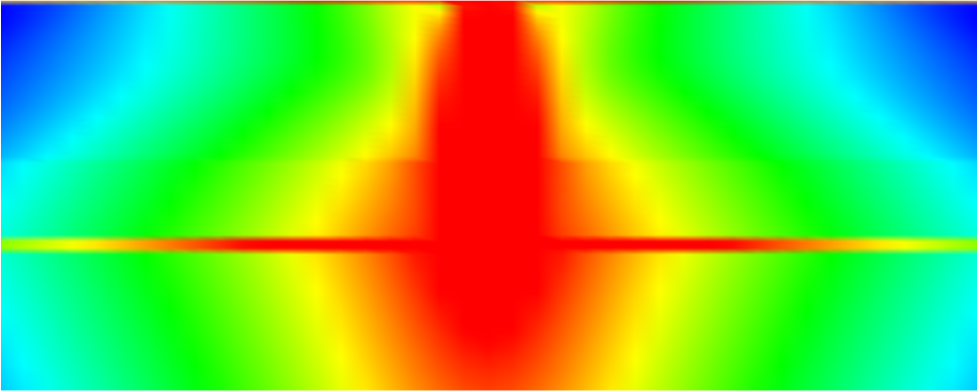
Offset versus Depth total electric field amplitude grid
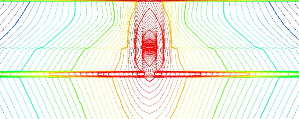
Offset versus Depth total electric field amplitude contours
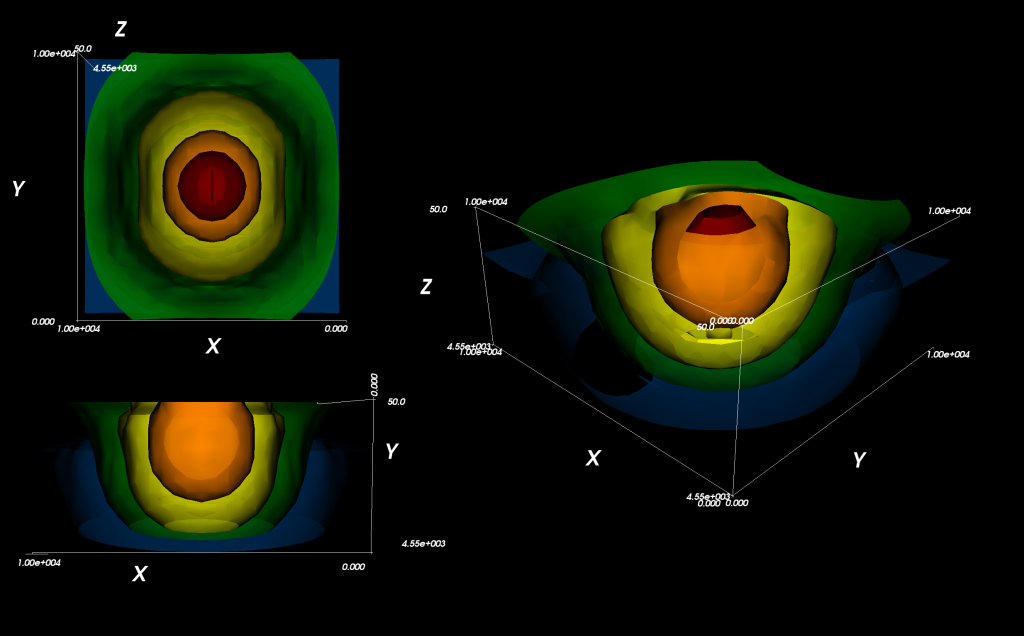
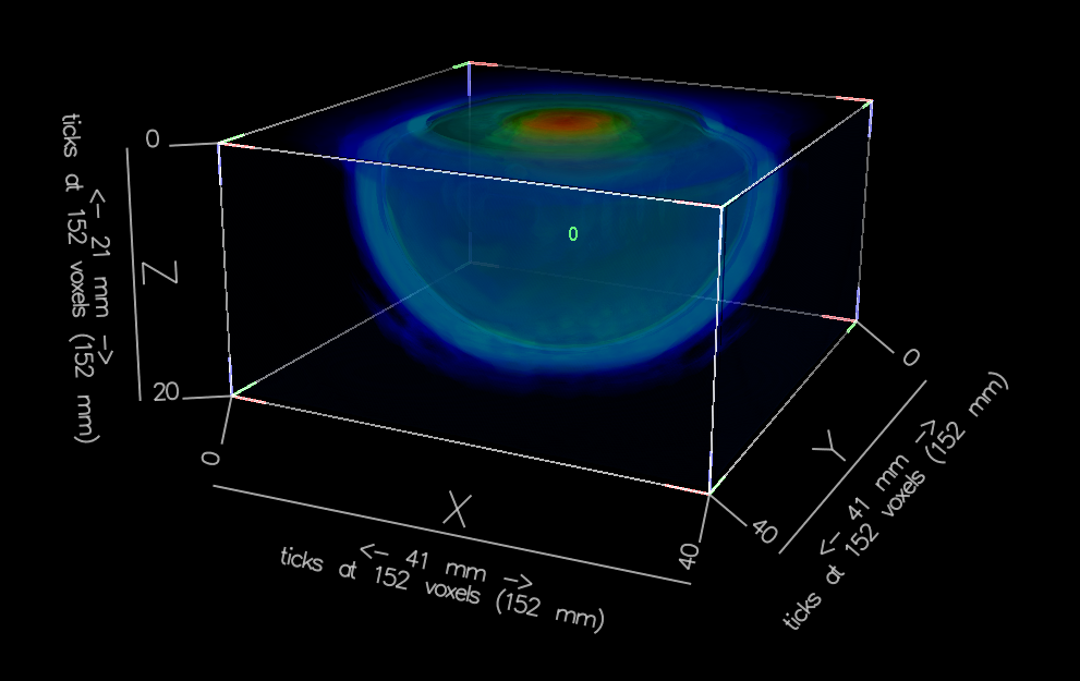
Isosurfaces
Isosurfaces represent a surface of scalar equipotential value and is the 3D contour. Much like 2D contours, multiple isosurfaces can clutter a visualisation. 2D contours can represent two variables and a scalar whilst isosurfaces can test three variables and a scalar. Two examples of isosurfaces can be seen below.
-
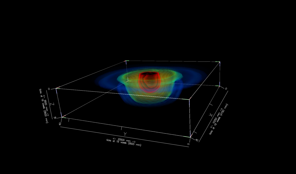
- Isosurface rendering in Drishti
-
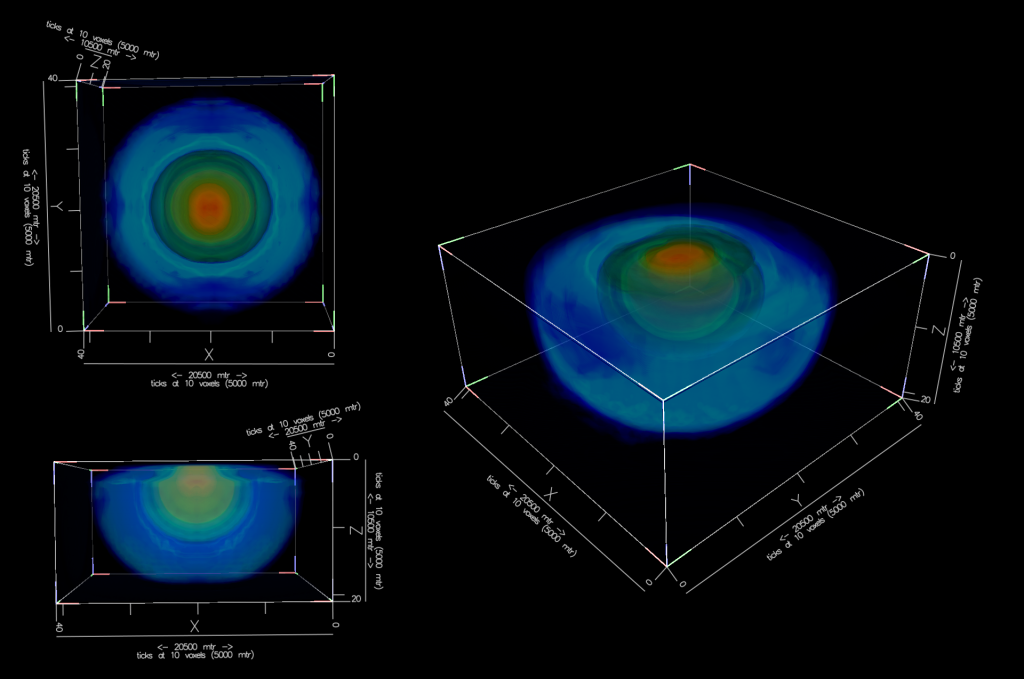
- Isosurface rendering in Drishti
-
- Isosurface rendering in Mayavi
-
- Isosurface rendering in Drishti
-
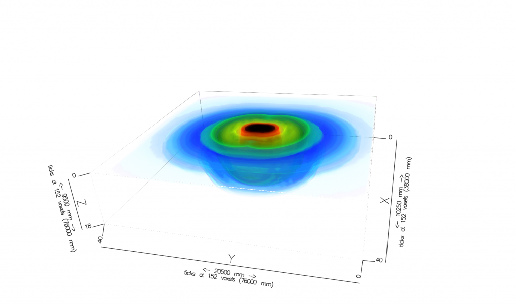
- Isosurface rendering in Drishti
Vector Glyphs
A vector glyph is a 3D object containing geometric and magnitude information. In mathematics, they are essentially Euclidean, geometric or spatial vectors. Vectors are not commonly utilised in geophysical visualisation. HoweverWeidelt (2007) and Harris and Pethick (2008) offer some examples of 2D vector representation. 3D vector glyph can be easily applied to represent electromagnetic fields. Vector algebra is used to compute various pieces of information including, Poynting, current density vector and scattered, total and background responses.
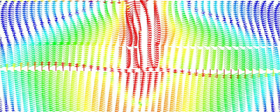
Electric field XY Amplitude Vectors in the offset versus depth plane
Polarisation Ellipses
Multiple attributes can be visualized using vectors as the direction, scale, length and color can all contain attributes. As a result, vectors can represent scalar amplitude, scalar phase, time amplitude vector, real and imaginary vectors (See Videos 1-2 and 1-3). It is difficult to use vector glyphs to display field paths as they only visualize the field direction at a point in time. (Ax, Ay and Az) at a several times are computed and stored in an array. A complete time series must be computed from the amplitude and phase by using the transmitter waveform, in the case of the frequency domain MCSEM method it is the vector addition of multiple sinusoidal
functions, for all Cartesian directions. The amplitude for a given time can be computed by Equation 1:
Equation 1 : 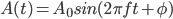
where,
 - Amplitude at time
 - Total amplitude =
 - Phase
 - Frequency
- Time 
As seen in Figure 2 the completed array of amplitude over the whole cycle forms the points of an ellipse. This ellipse is best represented by a polygon. This polygon is created from the array of stored time amplitude vectors. These amplitudes are then normalised by the maximum
amplitude to transform the ellipse into a unit ellipse centred at point P(0,0,0),
Equation 2 : 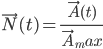
or more precisely,
Equation 3 : 
where,
 - Normalised amplitude vector at time
 − Maximum total amplitude over whole period
To visualise the ellipse, the ellipse needs to be scaled to reasonable proportions and positioned. The ellipse is scaled by multiplying the normalised values by the ellipse size. This ellipse size can be either a constant (i.e., single ellipse size) or variable (i.e., scaled by amplitude). The scaled vector can be simplified as,
Equation 4 : 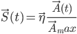
where,
- Scaled normalised amplitude vector at time
 - Scaling factor
The ellipse is then positioned into the final cartesian co-ordinates. It’s final position depends on the user-selected geometry (i.e., receiver location, transmitter location, transmitter-reciver midpoint etc. . . ),
Equation 5 : 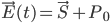
where,
 - Final ellipse vertex co-ordinate at time
 − Centre of ellipse (determined by user-selected geometry)
To clarify the formulation of polarisation ellipses Video 3-16 shows the formulation of a three-dimensional electric field ellipse. This representation can be used to establish the direction of maximum amplitude and can be used to infer the generalised path of electric and magnetic fields. Polarisation ellipses also contain phase information phase for each of the components. These polarisation ellipse polygons are stored as vertex buffers to improved visualisation speed.
The schematic demonstrating the formulation of a polarisation ellipse. Electromagnetic field vectors vary in amplitude over time. Figure A highlights twelve 2D electric field vector orientations. The complete elliptical rotation of the field can be encapsulated by a polygon (see Figure B). The polarisation ellipse representation contains amplitude, and phase and polarisation directions. Polarisation ellipses can also be used to visualise the 3D magnetic, electric and Poynting vector fields to contrast the electric and magnetic fields or show the differences in attributes of the scattered, total and layered responses.
The formation of an electric field ellipse